绘图

单变量函数

在 MATLAB 中绘图包含下面三个步骤：

定义函数
指定要绘制的函数图形的值范围
调用 MATLAB 的 plot(x, y)函数

当指定函数的值范围时，我们必须告诉 MATLAB 函数使用的变量的增量。使用较少的增量可以使得图形显示更加平滑。如果增量较小，MATLAB 会计算更多的函数值，不过通常不需要取得那么小。我们用一个简单的例子来看看如何做。

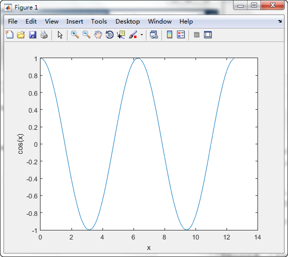
我们绘制 0≤x≤10 之间的 y = cos(x)的图形。绘制之前，我们要定义这个区间并告诉
MATLAB 我们所使用的增量。区间使用方括号[]以下面的形式定义：
[ start : interval : end ]

例如，如果我们要告诉 MATLAB 在 0≤x≤10 上以 0.1 的增量（间隔）递增，我们输入：

[0:0.1:10]

用赋值运算符给这个范围内的变量一个名称，也用这种办法告知 MATLAB 相关变量和我们要绘制的函数。因此，要绘制 y = cos(x)，我们输入下面的命令：

1 2	>> x = [0:0.1:4*pi]; >> y = cos(x);

注意我们每行都以分号“;”结尾，记住，这会抑制 MATLAB 输出。你不会想让 MATLAB
在屏幕中间输出一大串 x 值，因此使用了分号。现在我们可以输入下面的命令绘图了：
>> plot(x, y), xlabel('x'), ylabel('cos(x)')

fplot

上面的例子只是简单的提供了一种图形曲线画法函数，然而当我们遇到需要多个包含变量的函数进行乘除运算时，就会出现：

>> t = [0:0.02:4];
>> f = exp(-2*t)*sin(t);
Error using  * 
Inner matrix dimensions must agree.
 
>> f=2*sin(t);
>> f=2*x*sin(t);
Error using  * 
Inner matrix dimensions must agree.

为什么会出现这种情况呢？在Matlab中，x是一个[0:0.02:4]的矩阵，同样sin(x)也是一个矩阵。*是矩阵乘法operator。x是一个长度为200的矩阵，sin(x)也是如此。也就是说，x和sin(x)都是1*200的矩阵，这在矩阵乘法中显然是无法进行的。所以提醒Inner matrix dimensions must agree

此时我们可以使用dot乘，对应元素分别相乘。

exp(-2*x).*sin(x)

或者使用fplot函数：

>> help fplot
 fplot   Plot function
    fplot(FUN,LIMS) plots the function FUN between the x-axis limits
    specified by LIMS = [XMIN XMAX]. Using LIMS = [XMIN XMAX YMIN YMAX]
    also controls the y-axis limits. FUN(x) must return a row vector for
    each element of vector x. For example, if FUN returns
    [f1(x),f2(x),f3(x)] then for input [x1;x2] FUN should return
 
       [f1(x1) f2(x1) f3(x1);
        f1(x2) f2(x2) f3(x2)]
 
    fplot(FUN,LIMS,TOL) with TOL < 1 specifies the relative error
    tolerance. The default TOL is 2e-3, i.e. 0.2 percent accuracy.
 
    fplot(FUN,LIMS,N) with N >= 1 plots the function with a minimum of N+1
    points. The default N is 1. The maximum step size is restricted to be
    (1/N)*(XMAX-XMIN).
 
    fplot(FUN,LIMS,'LineSpec') plots with the given line specification.
 
    fplot(FUN,LIMS,...) accepts combinations of the optional arguments
    TOL, N, and 'LineSpec', in any order.
    
    [X,Y] = fplot(FUN,LIMS,...) returns X and Y such that Y = FUN(X). No
    plot is drawn on the screen.
 
    fplot(AX,...) plots into AX instead of GCA.

fplot 为你产生尽可能精确的的图象，同时它也帮助我们绕过像这样的错误。调用 fplot 的形式如

fplot('function string', [xstart, xend])

参数 function string 告诉 fplot 你所要绘制的图象函数，而 xstart 和 xend 定义了函数的区间。

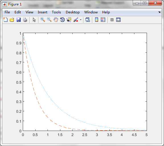
>> fplot('exp(-2*t)*sin(t)',[0, 4]), xlabel('t'), ylabel('f(t)'),title('阻尼弹力')

多个函数

Matlab支持多个函数在一张图表中显示：

>> t = [0:0.01:5];
% 接着我们定义两个函数
>> f = exp(-t);
>> g = exp(-2*t);

plot(t,f,t,g,'--')

上面的例子告诉Matlab要绘制 f(t)和 g(t)函数，并且第二个函数曲线使用虚线。

实线 ‘-‘
虚线 ‘–’
虚点线 ‘-.’
点线 ‘:’

>> plot(t,f,':',t,g,'--')

添加图例

专业的图象总是附有图例，告诉读者某个曲线是什么。在下面的例子中，假设我们要绘制两个表示势能的函数，它们由双曲三角函数 sinh(x)和 cosh(x)定义，定义域为 0≤x≤2。首先我们定义x：

>> x = [0:0.01:2];

现在我们定义这两个函数，在 MATLAB 中把函数称为 y 并不是什么不可思议的事，所以我们把第二个函数称为 z，因此有：

1 2	>> y = sinh(x); >> z = cosh(x);

legend 命令用起来很简单。只需把它加在 plot(x,y)命令后面，并用单引号把要添加为图例的文本引起来。在这个例子中我们有：

legend('sinh(x)','cosh(x)')

我们只需把这一行添加到 plot 命令后面。在这个例子中，我们还包含 x 和 y 标签，第一条曲线用实线而第二条曲线用虚点线：

1	>> plot(x,y,x,z,'-.'), xlabel('x'), ylabel('Potential'), legend('sinh(x)','cosh(x)')

颜色设置

相比其他类似的开发工具，Matlab画图是也同样支持设置图像颜色。

plot(x,y,'r',x,z,'b--')

上面的代码代表第一个函数为红色，第二个以虚线填充的函数为蓝色。

白色 w
黑色 k
蓝色 b
红色 r
青色 c
绿色 g
洋红 m
蓝色 y

设置坐标比例

axis命令可以设置绘图范围。通过用下面的方式调用 axis 命令：

axis ([xmin xmax ymin ymax])